How to Optimize Amazon Redshift for Analytics Without Overprovisioning

Distribution keys determine how Redshift spreads rows across compute nodes, and a poor choice here is the single most common cause of slow joins. When two large tables joined on customer_id live on different nodes, Redshift redistributes one of them at query time — a network-heavy operation that shows up in EXPLAIN plans as DS_DIST_ALL_INNER or DS_BCAST_INNER.

Redshift offers four distribution styles. KEY distributes rows by the values of a specified column, so rows with the same key land on the same node. EVEN distributes rows round-robin regardless of content. ALL copies the entire table to every node (useful for small dimension tables under roughly 3 million rows). AUTO lets Redshift choose and adjust the style based on observed query patterns.

When to Set a Manual DISTKEY

If your workload has a dominant join pattern — say, most reports join on account_id or product_id — setting that column as the DISTKEY eliminates redistribution for those joins. The trade-off: joins on other columns may still require shuffling. According to AWS’s own table design documentation, the best DISTKEY candidate is a column that appears frequently in JOIN conditions and has high cardinality with even distribution of values (Amazon Redshift best practices for designing tables).

A column with severe skew — where a handful of values account for most rows — makes a bad DISTKEY. Redshift will pile data onto a few slices, and those slices become bottlenecks during scans and joins. Check skew with SVV_TABLE_INFO’s skew_rows column; anything above 1.4 deserves investigation.

When AUTO Distribution Works Well Enough

Automatic table optimization (ATO) observes query patterns and adjusts distribution and sort keys in the background. For teams that don’t have a DBA reviewing table design regularly, ATO is a reasonable default. It won’t always pick the optimal key for complex multi-table joins, but it prevents the worst outcomes. You can enable it on existing tables with ALTER TABLE <table_name> ALTER DISTSTYLE AUTO.

For teams already running heavy workloads, ATO should be treated as a starting point, not a replacement for manual review. Cross-reference Redshift Advisor recommendations with your actual EXPLAIN plans before accepting all automated changes. General data modeling patterns that reduce query time apply here: a well-designed star schema with clear fact-dimension relationships gives ATO much better signal than a flat denormalized dump.

Sort keys define the physical order of rows on disk. When a query filters on a sort key column, Redshift uses zone maps — metadata that tracks the minimum and maximum values in each 1 MB block — to skip blocks entirely. A well-chosen sort key on a time-series table can reduce scan volume by an order of magnitude for queries filtering on recent dates.

Compound sort keys sort rows by the first column, then by the second within groups of the first, and so on. They work well when queries consistently filter on the leading column. A table with COMPOUND SORTKEY (event_date, region) benefits heavily from WHERE event_date > ‘2026-01-01’, but gets almost no benefit from WHERE region = ‘EU’ alone, because zone map elimination only kicks in on the leading column.

Interleaved sort keys give equal weight to each column in the key, which helps when queries filter on different columns at different times. The cost is higher maintenance: interleaved keys require more frequent VACUUM REINDEX operations to stay effective, and those operations are resource-intensive.

Practical Sort Key Selection

For most analytics tables, compound sort keys starting with a date column (event_date, created_at, transaction_date) cover the majority of queries. If your team runs both time-filtered and dimension-filtered queries with similar frequency, consider whether two separate tables or a materialized view might serve the workload better than an interleaved key. Materialized views in Redshift auto-refresh and can pre-aggregate or pre-join data for the secondary access pattern without the VACUUM REINDEX overhead.

If your Redshift queries are slowing down and your team isn’t sure whether the problem is table design, workload contention, or both — an architecture review with engineers who’ve tuned Redshift at production scale will narrow the scope faster than trial-and-error. Schedule a Redshift optimization assessment.

Redshift’s columnar architecture stores each column separately, and compression encoding determines how efficiently that storage is used. Better encoding means smaller blocks, fewer I/O operations per query, and more data fitting into memory. The effect compounds on wide tables — a table with 80+ columns and no explicit encoding will scan significantly more data than the same table with appropriate compression applied.

Since 2021, Redshift’s ATO also covers column compression: tables created with ENCODE AUTO let the engine pick and adjust encodings over time. For existing tables that predate this feature, run ANALYZE COMPRESSION <table_name> to get AWS’s recommendation for each column. Applying those recommendations typically requires rebuilding the table (CREATE TABLE AS SELECT or deep copy), which is disruptive but often produces noticeable scan-time reductions.

One specific caution: avoid compressing the leading sort key column. AWS’s prescriptive guidance explicitly recommends leaving the sort key column with RAW (no compression) encoding, because compression on that column can interfere with zone map effectiveness and hurt scan pruning.

amazon-redshift-optimization-sequence

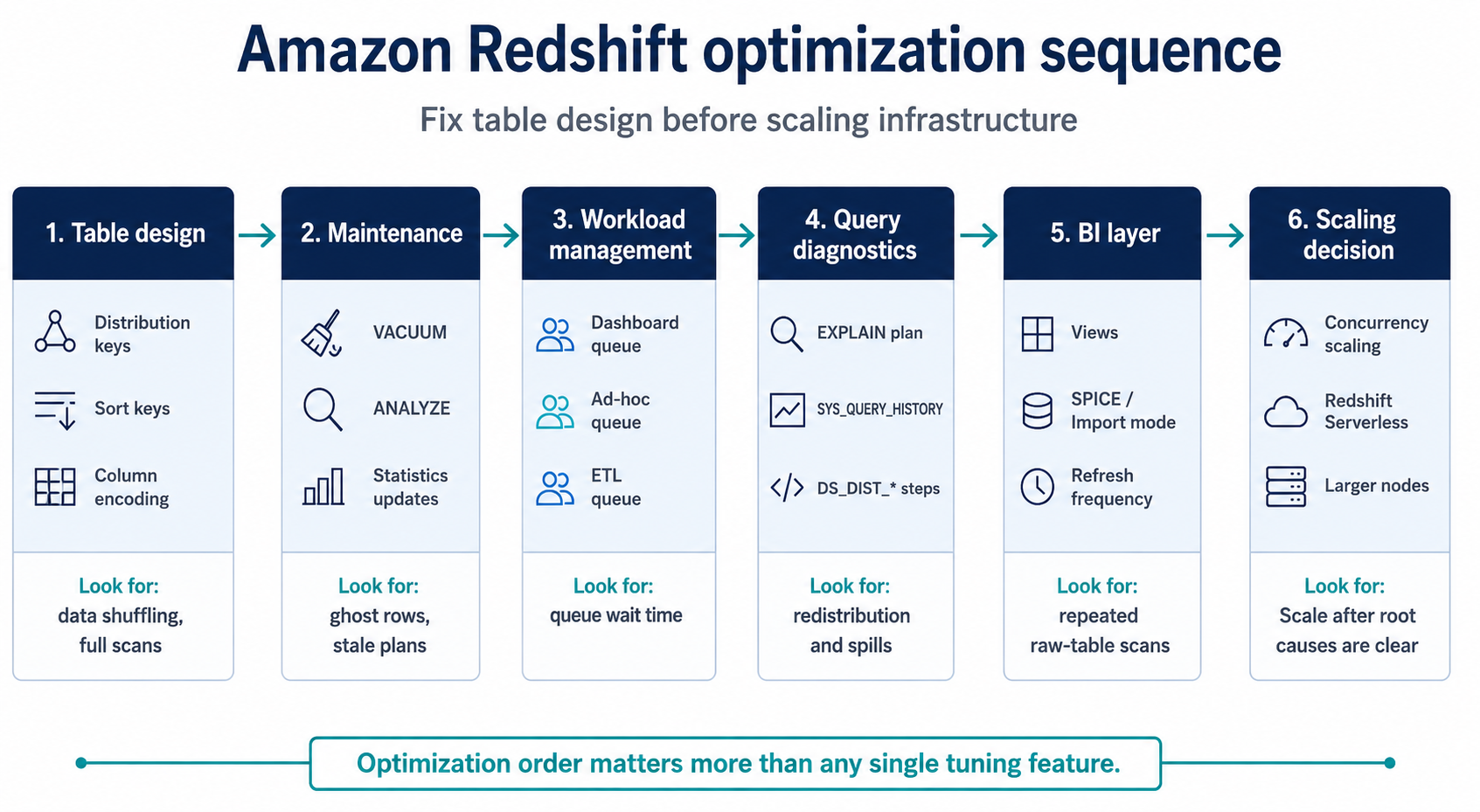
Redshift performance tuning works best as a sequence: fix table design first, clear maintenance debt, separate workloads with WLM, diagnose query behavior, and scale only after the core issues are visible.

Workload Management (WLM) controls how Redshift allocates memory and concurrency slots across queues. Without WLM tuning, a single expensive analytical query can consume all available slots, blocking lightweight dashboard refreshes from executing until it finishes. This is one of the most reported frustrations from BI teams sharing a Redshift cluster across scheduled reports, ad-hoc analysis, and ETL loads.

Manual WLM vs. Automatic WLM

Redshift’s automatic WLM dynamically adjusts memory allocation and concurrency based on query demands. For workloads that are unpredictable or still being characterized, auto WLM is a reasonable starting point. Manual WLM gives explicit control: you define separate queues for ETL, dashboards, and ad-hoc queries, each with its own memory percentage and concurrency limit.

The practical pattern that works in most mid-market environments: three queues. A high-priority queue with 2–3 concurrency slots and 40–50% memory for scheduled dashboards and reports. A medium-priority queue for ad-hoc analyst queries. A low-priority queue for data loads and maintenance jobs, configured to run when the other queues are idle.

Since January 2026, Redshift Serverless supports queue-based query resource management with per-queue monitoring rules. Teams on Serverless can now set query timeout thresholds and resource limits per queue — a capability that previously required provisioned clusters with manual WLM. This narrows the operational gap between Serverless and provisioned for production analytics workloads.

Concurrency Scaling: What It Solves and What It Doesn’t

Concurrency scaling adds temporary clusters to handle read-query bursts. It helps when query volume spikes beyond what the main cluster can handle — for example, when 50 users open dashboards simultaneously at 9 AM. It does not help when individual queries are slow because of poor table design or missing sort keys. Turning on concurrency scaling for a cluster whose underlying tables need redesign is like adding lanes to a road with a broken bridge: the throughput bottleneck hasn’t moved.

Redshift does not automatically reclaim storage from deleted or updated rows. These “ghost rows” accumulate over time, inflating scan volume and degrading sort order. VACUUM reclaims space and re-sorts rows; ANALYZE updates the statistics the query optimizer uses to build execution plans. Skipping both is a common cause of gradual performance degradation that teams attribute to data growth when the real issue is maintenance debt.

VACUUM Types and When to Use Each

VACUUM FULL re-sorts the entire table and reclaims all deleted space. It’s the most thorough option, but also the most resource-intensive — avoid running it during business hours on large tables. VACUUM DELETE ONLY reclaims space without re-sorting, which is faster and sufficient for tables where the sort order hasn’t drifted. VACUUM SORT ONLY re-sorts without reclaiming space. VACUUM REINDEX rebuilds interleaved sort key indexes, and is necessary only for tables using interleaved keys.

A practical maintenance schedule for most mid-market clusters: run VACUUM DELETE ONLY on heavily updated tables nightly or after each major ETL load. Run VACUUM FULL on fact tables weekly during a low-traffic maintenance window. Run ANALYZE after any load that adds more than a few percent of new rows. If you’re on Redshift Serverless, note that Redshift handles some background maintenance automatically, but explicit ANALYZE after large loads still improves optimizer accuracy.

EXPLAIN, STL_ALERT_EVENT_LOG, SYS_QUERY_HISTORY, and SVL_QLOG — expose the internal mechanics: how many rows were scanned vs. returned, whether data was redistributed across nodes, and whether the query hit disk instead of memory.

Three Patterns That Signal Tuning Opportunities

A high scanned-to-returned row ratio (check EXPLAIN output for sequential scans on large tables) usually means missing or misaligned sort keys. Zone maps can’t skip blocks if the filter column doesn’t match the sort key. Network redistribution steps (DS_DIST_*) in the EXPLAIN plan point to distribution key mismatches between joined tables. Temporary table spills to disk (visible in STL_ALERT_EVENT_LOG with the “very selective filter” or “missing statistics” alerts) often indicate that ANALYZE hasn’t been run recently.

AWS’s query design best practices recommend specific structural adjustments: avoid SELECT * and list only needed columns, add redundant predicates on joined tables to help the optimizer skip blocks, use CASE expressions instead of multiple passes over the same table, and prefer subqueries over joins when the filtering table returns fewer than about 200 rows (Amazon Redshift best practices for designing queries).

BI Tool Integration: Where Dashboard Design Becomes a Cluster Problem

Even a well-tuned cluster suffers when BI tools generate inefficient SQL. Common issues include dashboards that run SELECT * against raw fact tables instead of pre-built views, auto-refresh intervals set to 30 seconds when the data only updates hourly, and filters that the BI tool applies client-side instead of pushing down to SQL.

Amazon Quick Suite’s SPICE engine caches data locally, which offloads repeated queries from Redshift. Power BI can use DirectQuery or Import mode — Import mode reduces Redshift load but introduces data staleness. Both tools benefit from connecting to Redshift views rather than raw tables, because views enforce consistent business logic and reduce the surface area of queries hitting the cluster. Teams evaluating which BI tool fits their AWS stack can compare the trade-offs in Bluepes’s Power BI vs Amazon Quick Suite comparison.

Redshift Serverless removes cluster sizing and node management, but table design decisions — distribution keys, sort keys, encoding — still matter exactly as much. A poorly designed table scans the same excess data whether it’s running on a provisioned ra3.xlarge cluster or a Serverless workgroup. The difference is how you pay for that waste: on provisioned clusters, you pay for idle nodes; on Serverless, you pay per RPU-second of compute consumed.

AWS announced new Graviton-based RG instances in May 2026, which run data warehouse workloads up to 2.2x faster than RA3 instances at 30% lower price per vCPU (Amazon Redshift RG instances announcement). For provisioned cluster users, this changes the cost-performance math. But the optimization sequence remains the same: fix table design first, tune WLM second, and scale hardware only after the first two are addressed.

On the cost side, Redshift Serverless now offers 3-year reservations with up to 45% savings on committed RPU capacity. For teams whose Redshift usage has stabilized, reserving baseline RPUs and handling peaks with on-demand pricing keeps costs predictable. Teams building ETL or real-time data pipeline architectures feeding into Redshift should factor these cost models into their pipeline design from the start.

Key Takeaways

• Distribution key mismatches cause cross-node data shuffling on every join — check EXPLAIN plans for DS_DIST_* steps before scaling hardware.
• Compound sort keys starting with a date column cover the majority of analytics query patterns and enable zone map block skipping.
• VACUUM and ANALYZE are not optional housekeeping — ghost rows and stale statistics are among the most common causes of gradual Redshift performance degradation.
• WLM queue separation prevents expensive ad-hoc queries from blocking time-sensitive dashboards and scheduled reports.
• Table design decisions affect Serverless cost directly: inefficient scans translate to higher RPU-second charges, not just slower responses.

The teams that get the most from Redshift tend to follow a consistent order: fix distribution and sort keys first, because they affect every query that touches the table. Run VACUUM and ANALYZE to clear accumulated maintenance debt. Then configure WLM queues so that workload contention doesn’t mask the improvements. Only after those three steps does it make sense to evaluate concurrency scaling, Serverless migration, or larger node types.

Skipping ahead to infrastructure changes before addressing table design produces temporary relief and recurring cost increases. The physical design of your tables is the foundation — everything else is built on top of it.

If your analytics team needs an external review of Redshift table design, WLM configuration, or cluster sizing for an AWS-native BI stack, Bluepes’s data engineering and analytics services team can run a focused optimization audit and deliver concrete recommendations within two weeks. Start with a Redshift assessment.